Problem Set 6
Due 11/6/26
Places highlighted in yellow denote where you need to take a screenshot or write a response. Steps highlighted in blue are ones you already did in Problem Sets 1–5 (look back at those if you need help).
Data
Instructor Demo: CHAIR vs. SCRAMBLED pictures (same file)
Student Independent Work to Turn In: FACE vs. HOUSE pictures
Overview
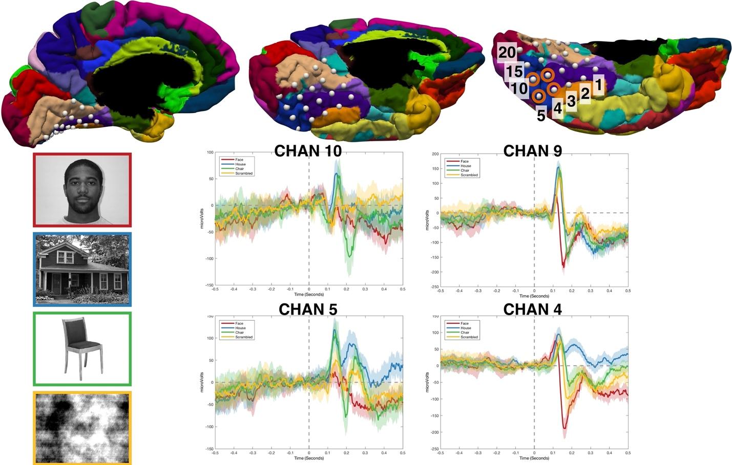
Overview: This week we will work with a new kind of data: ECoG (electrocorticography), recorded from electrodes placed directly on the surface of the brain. The study again involves the N170 response. The patient viewed pictures of faces, houses, chairs and scrambled images, one every 1.8 seconds, and pressed a button whenever the same picture appeared twice in a row (to stay attentive). Those button-press trials (labeled REPEAT) are left out of the analysis, which leaves 100 trials: 25 FACE, 27 HOUSE, 23 CHAIR and 25 SCRAMBLED. We only analyze the 20 electrodes (so1–so20) placed on the underside of the temporal lobe (the ventral temporal lobe, Figure 1). Of particular interest for this study is the fusiform gyrus, shown in purple.
You will compare FACE with HOUSE. The instructor demo runs the same steps on CHAIR vs. SCRAMBLED from the same file, so its results (channels, times) will be different from yours.
Figure 1
1)[0.4 pts] Set up the study in Brainstorm
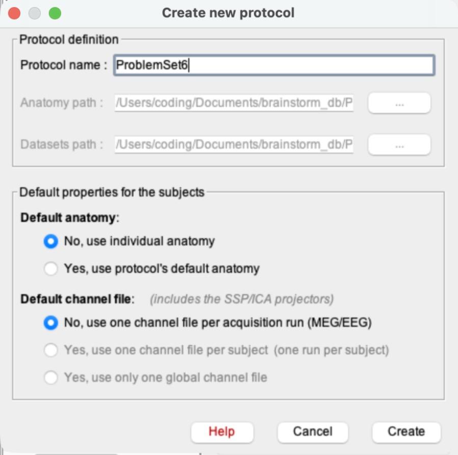
a)File > New protocol. Name it ProblemSet6.
b)This time, choose No for both defaults. Default anatomy: “No, use individual anatomy”. Default channel file: “No, use one channel file per acquisition run (MEG/EEG)” (the two “Yes” channel options are grayed out once you pick No for anatomy). Click Create.
Why “No” this time? In Problem Sets 1–5 you used Brainstorm’s template head and a standard EEG cap, because scalp electrodes sit in the same places on everyone. ECoG electrodes are placed on one patient’s own brain, so a template head would put them in the wrong place. The electrode positions saved in this data file are the right ones, which is also why you won’t use “Add EEG positions” in this problem set.
c)Switch the database view to the middle icon (functional data sorted by subjects), as in PS1 and PS5.
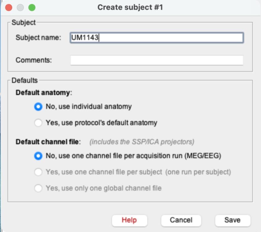
d)Right-click ProblemSet6 > New subject. Name it UM1143. Both defaults already say No (copied from the protocol). Click Save.
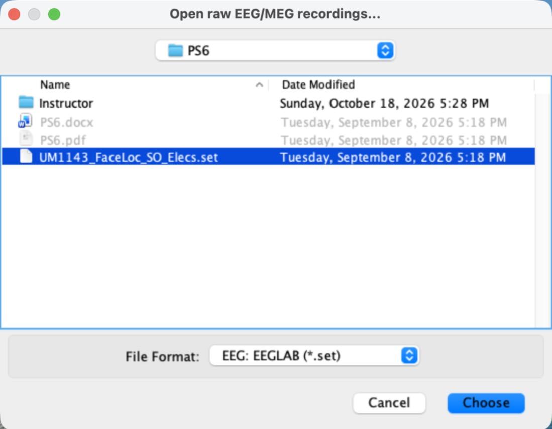
e)Right-click UM1143 > Review raw file. Change the File Format to “EEG: EEGLAB (*.set)” and select UM1143_FaceLoc_SO_Elecs.set.
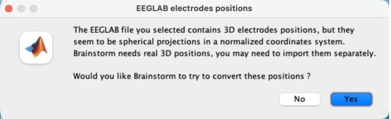
f)A pop-up asks whether Brainstorm should try to convert the electrode positions. Click No.
You don’t need to edit the channels this time: these 20 electrodes are not a standard EEG cap, and they are already set to type EEG.
g)Double-click “Link to raw file” to plot the raw recording in Column mode. Set the montage to Average reference (Display configuration button > Montage > Average reference) and the Duration to 20 s in the Record tab, as in PS3 and PS4. Scroll to a part of the recording with events. Take a screenshot of the time-series plot.
h)Can you find periods in the recording that look like the eye-blink artifacts you saw in PS3 and PS4? Why or why not?
2)[0.6 pts] Create ERPs
a)Close the plot. Right-click “Link to raw file” > Import in database.
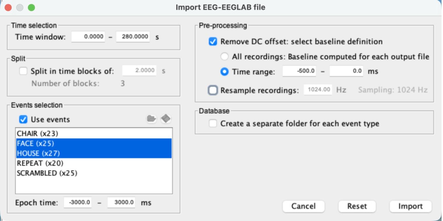
i)Check “Use events” and select FACE and HOUSE (Cmd-click on a Mac, Ctrl-click on Windows).
ii)Set the Epoch time to -3000 to 3000 ms.
iii)Check “Remove DC offset”, choose “Time range”, and set it to -500 to 0 ms.
iv)Leave “Create a separate folder for each event type” unchecked. Your settings should match the screenshot for step 2a (camera icon). Click Import.
You should get two groups of single trials: FACE (25 files) and HOUSE (27 files).
b)Select both groups, FACE (25 files) and HOUSE (27 files) (Cmd-click), and drag them into “Files to process” (Process1). It should say Data [52].
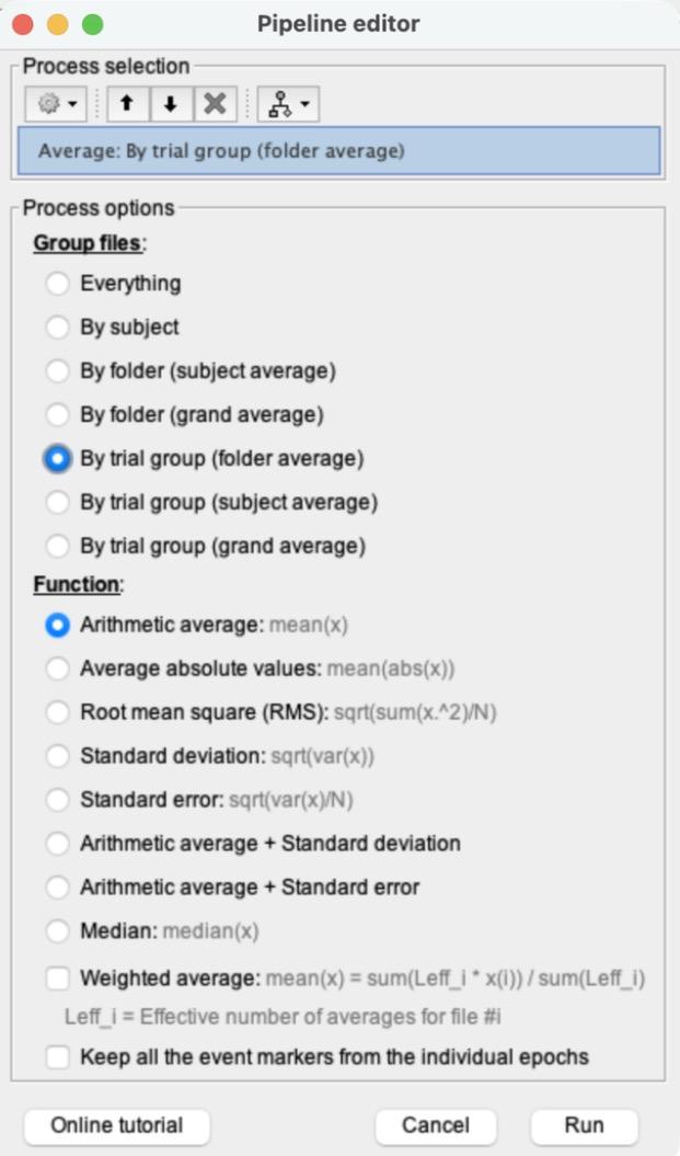
i)Click RUN > gear icon > Average > Average files. Choose “By trial group (folder average)” and “Arithmetic average”, then click Run.
This creates “Avg: FACE (25 files)” and “Avg: HOUSE (27 files)”.
c)Double-click Avg: FACE and Avg: HOUSE to plot both, and put both in Column mode.
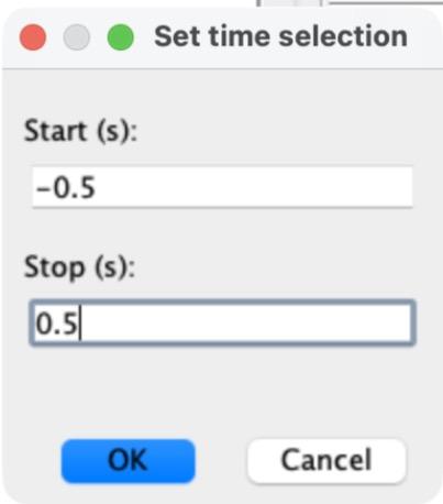
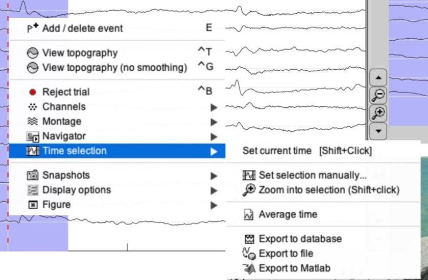
i)Set each plot to -500 to 500 ms: right-click inside the plot > Time selection > Set selection manually…, type -0.5 and 0.5 (seconds) and click OK. Then right-click again > Time selection > Zoom into selection.
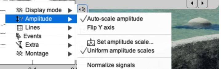
ii)Give both plots the same amplitude scale: click the Display configuration button on the right edge of the plot > Amplitude > Set amplitude scale…, type 200 and press Enter. Do this for both plots.
iii)Click in either plot at about 170 ms to drop the time cursor there (the time shows in the top left corner). Both plots move together.
iv)Take a screenshot of both plots.
d)Select both Avg: FACE and Avg: HOUSE (Cmd-click) > right-click > 2D Layout: EEG.
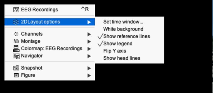
i)Right-click inside the new plot > 2DLayout options > Set time window…, and enter -500 and 500 (ms). Otherwise each channel shows the whole -3 to 3 s and the N170 is a tiny wiggle.
ii)Right-click > Channels > Display labels. Zoom in by scrolling, click and drag to recenter, and use the vertical arrow buttons to change the amplitude if needed (as in PS2).
iii)Find a channel with a typical N170 response (a large negative peak between about 150 and 200 ms, bigger for FACE than for HOUSE) and take a screenshot. Draw an arrow to the N170 on your screenshot.
e)How many complete trials are captured in this epoch? Note that here an epoch spans from -3 s to +3 s relative to a stimulus onset, and that a stimulus was presented every 1.8 s.
3)[0.7 pts] Create a difference wave between the ERPs
a)Compute the difference wave Avg: FACE − Avg: HOUSE, as in PS5 step 6: click “Process2”, drag Avg: FACE into Files A and Avg: HOUSE into Files B, then click RUN > gear icon > Difference > Difference: A-B > Run. This creates “Avg: FACE (25 files) - Avg: HOUSE (27 files)”.
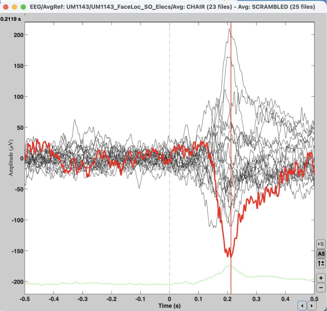
b)Double-click the difference wave to plot it in Butterfly mode and set it to -500 to 500 ms (as in step 2c.i). Click the line with the strongest (most negative) N170 difference to highlight it in red, then click at the bottom of that dip to place the time marker.
i)To see the channel’s name, press Enter with the line highlighted: a new plot opens with just that channel (as in PS1), and its name is in the box at the top right. Close it when you’re done.
ii)Take a screenshot of the butterfly plot with the time marker visible in the top left, and say which electrode has the strongest response and at what time point (in ms).
Instructor demo (CHAIR − SCRAMBLED, so14 highlighted). Your plot for FACE − HOUSE will look different.
c)Why does this channel have a strong N170 response? (Hint: look up where the channel is on the electrode map in Figure 1, available through this step’s camera icon. Several channels may show a strong response; you only need to report one of them.)
4)[0.7 pts] Independent t-test on single trials, with FDR correction
a)Clear the Files A and Files B panels (right-click inside each > Clear list).
b)Drag the FACE (25 files) group of single trials (not the Avg) into Files A and HOUSE (27 files) into Files B. The panels should say Data [25] and Data [27].
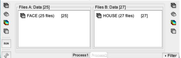
c)Click RUN > gear icon > Test > Parametric test: Independent. Type EEG in “Sensor types”, leave “Average selected time window” unchecked, and keep “Student’s t-test (equal variance)” and “Two-tailed”. Click Run.
Why independent? Every FACE trial and every HOUSE trial is a separate presentation, so the two groups of trials are independent of each other. (In PS5, the same 10 people contributed to both FACE and CAR, which is why that test was paired.)
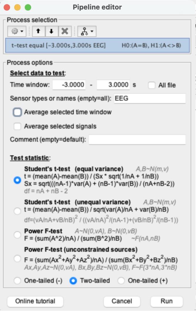
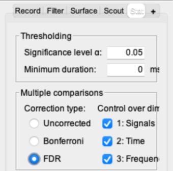
d)Double-click the new “t-test equal [-3.000s,3.000s EEG]: FACE (25) vs. HOUSE (27)” file to plot it. In the main Brainstorm window, open the Stat tab, set Multiple comparisons to “FDR”, and check that the significance level α is 0.05. (In PS5 you set it to Uncorrected, and Brainstorm remembers that, so you need to switch it.)
What FDR does: this t-test was run separately for every electrode at every time point: 20 channels × 6,145 time points = 122,900 tests. Without a correction (α = 0.05), about 1 in 20 tests can come out “significant” just by chance, which here could be thousands of false alarms. FDR (false discovery rate) correction ranks all the p-values and picks a stricter cutoff, so that among all the points it calls significant, no more than about 5% are expected to be false alarms. Here the cutoff becomes about p < 0.002 instead of p < 0.05. Switch between Uncorrected and FDR and watch the plot: most of the scattered blips before 0 ms disappear, while the large effect after the picture appears stays.
e)Set the plot to -500 to 500 ms (as in step 2c.i). Click the line with the biggest significance (the largest t-value, positive or negative) to highlight it, and click at its peak to place the time marker. Press Enter to see its name (as in step 3b). Take a screenshot of the FDR-corrected plot.
Instructor demo (CHAIR vs. SCRAMBLED, FDR, so14 highlighted). Your plot will look different.
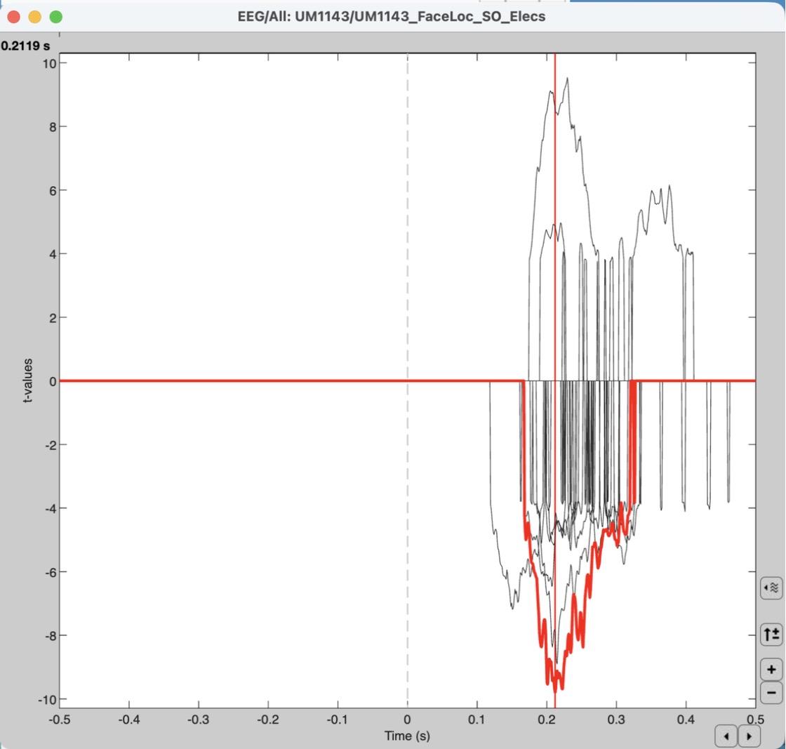
f)What’s the time point with the biggest significance? How does this compare to the one you found in step 3b?
g)Does the sign of the effect (positive or negative t) matter? (Hint: it doesn’t.) Think back to the lecture on the neurobiology of EEG signals, and explain why the polarity of the effect is irrelevant in the context of ECoG.
5)[0.7 pts] Spectral analysis: High-gamma band
a)Click “Process1” to switch back, and clear the “Files to process” list.
b)Drag the FACE (25 files) single trials into “Files to process”. Click RUN > gear icon > Frequency > Time-frequency (Morlet wavelets).
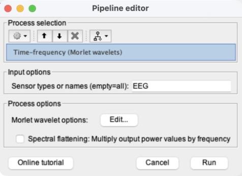
c)In “Sensor types or names”, replace “MEG, EEG” with EEG. Then click Edit… next to “Morlet wavelet options”.
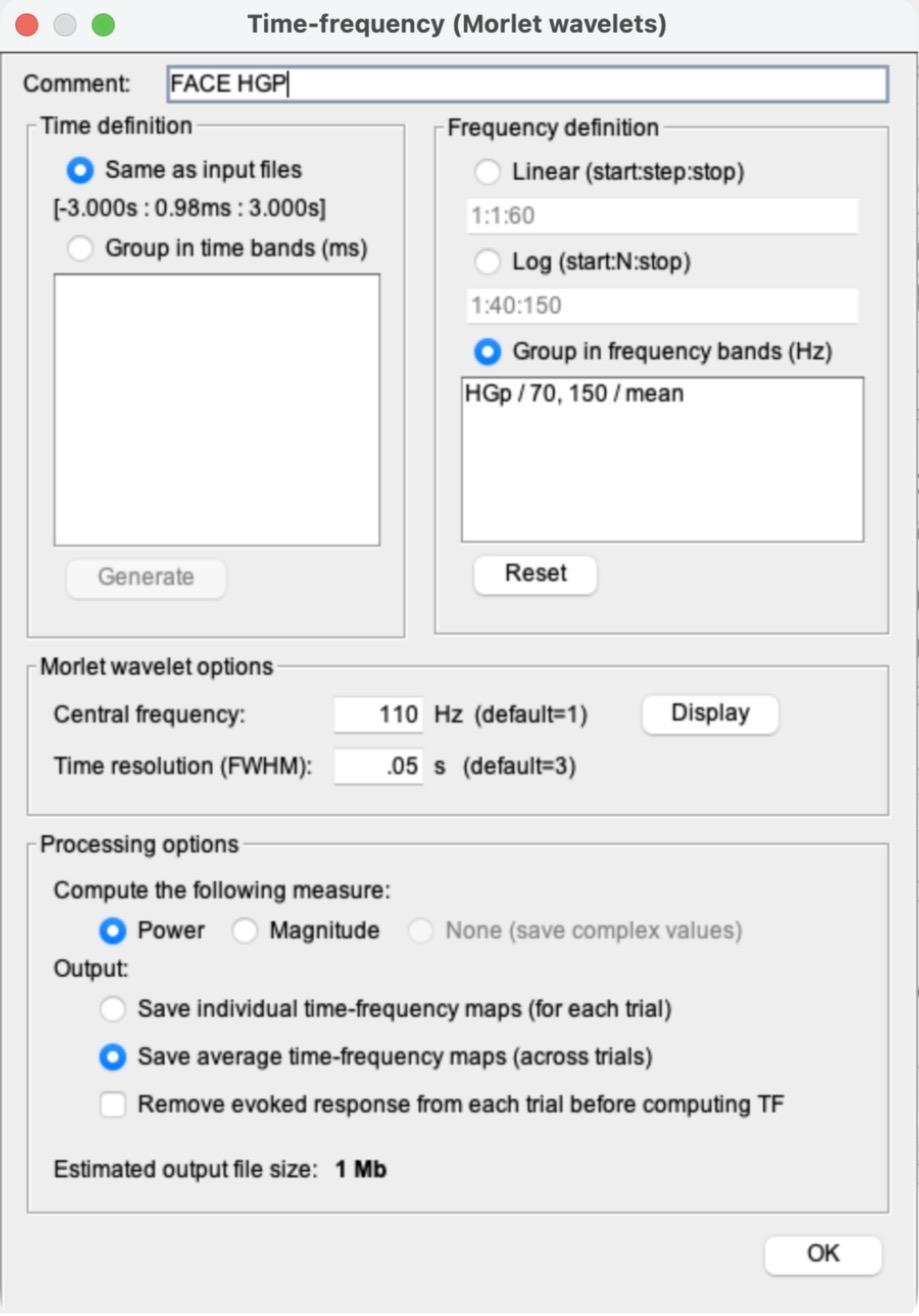
d)Use the settings in the screenshot (camera icon), in this order (Brainstorm rewrites the Comment when you change the frequency option, so the Comment goes last):
i)Frequency definition: select “Group in frequency bands (Hz)”. Delete everything in the box under it and type: HGp / 70, 150 / mean
ii)Morlet wavelet options: Central frequency 110 Hz and Time resolution (FWHM) 0.05 s.
iii)Processing options: “Power” and “Save average time-frequency maps (across trials)”.
iv)Comment at the top: FACE HGP. Then click OK.
e)Back in the Pipeline editor, do NOT check “Spectral flattening”. Click Run. A new file, “FACE HGP (EEG)”, appears.
f)Clear “Files to process”, drag in the HOUSE (27 files) single trials, and run the same process (RUN > Frequency > Time-frequency (Morlet wavelets) > Edit…). Brainstorm remembers the settings from the FACE run (check them against the screenshot for step 5d), but it resets the Comment to “Avg,Power,FreqBands”. Change only the Comment, to HOUSE HGP, click OK, and Run.
6)[0.5 pts] Create difference waves
a)Compute the HGP difference wave “FACE HGP − HOUSE HGP” the same way as step 3a: click “Process2”, clear Files A and B, drag FACE HGP (EEG) into Files A and HOUSE HGP (EEG) into Files B, then RUN > Difference > Difference: A-B > Run.
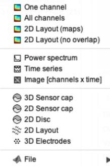
b)Right-click the new “FACE HGP (EEG) - HOUSE HGP (EEG)” file > Time series. It opens in Butterfly mode. Zoom in to about -0.5 to 0.5 s by scrolling (this plot doesn’t have the Time selection menu).
Tip: the axis numbers in this plot may be tiny in MATLAB 2026. That’s a display glitch and doesn’t affect this problem set.
c)Double-click the ERP difference wave from step 3 (Avg: FACE − Avg: HOUSE) to plot it in Butterfly mode, set to -500 to 500 ms.
d)Take a screenshot of both Butterfly plots from (b) and (c), side by side.
7)[0.4 pts] Written response
a)The channel with the strongest N170 response from step 3b should still be highlighted in the ERP difference plot (if not, click it again).
b)This highlights the same channel in the HGP difference plot.
c)Compare this channel in the HGP plot to the ERP plot, and explain what this means.
d)Some channels in the HGP plot have a negative difference (they dip below 0). What does a negative HGP difference imply?