Problem Set 5
Due 10/30/26
Instructor Demo: SUB_22, SUB_24, SUB_28, SUB_35, SUB_40 (_EDIT.set files)
Student Independent Work to Turn In: SUB_6 – SUB_15 (_EDIT.set files)
About these files:
the _EDIT files have already been cleaned for you. They are re-referenced to the average of all electrodes, high-pass filtered, and eye blinks were removed with ICA (like you did in PS4). Their event codes have also been renamed, so instead of numbers (1–40, 41–80, …) you will see FACE, CAR, sFACE (scrambled faces), sCAR (scrambled cars), Corr and Incorr (correct and incorrect responses).
In this problem set you will combine 10 subjects to do group-level statistics: average each subject’s trials, average across subjects, and test whether the N170 is more negative for faces than for cars.
1)[0.3 pts] Create a new protocol “ProblemSet5” and one subject for each data file
a)File > New protocol.
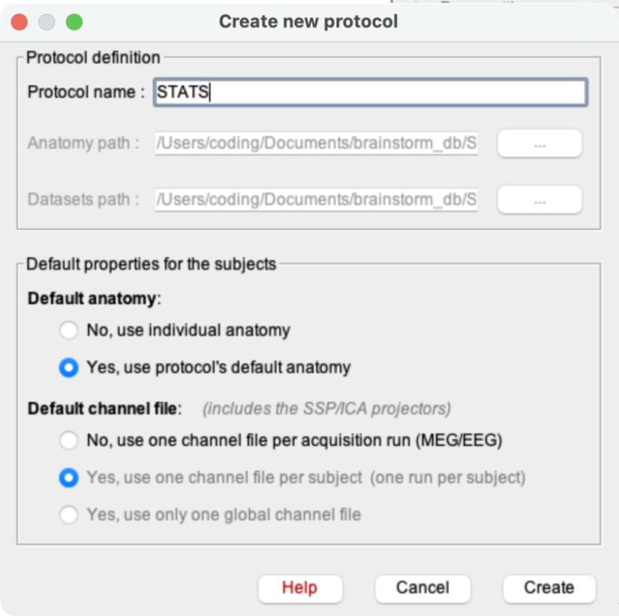
Name it ProblemSet5.
b)Default anatomy:
“Yes, use protocol’s default anatomy”. Default channel file: “Yes, use one channel file per subject (one run per subject)”. Click “Confirm” on the warning that pops up, then click Create.
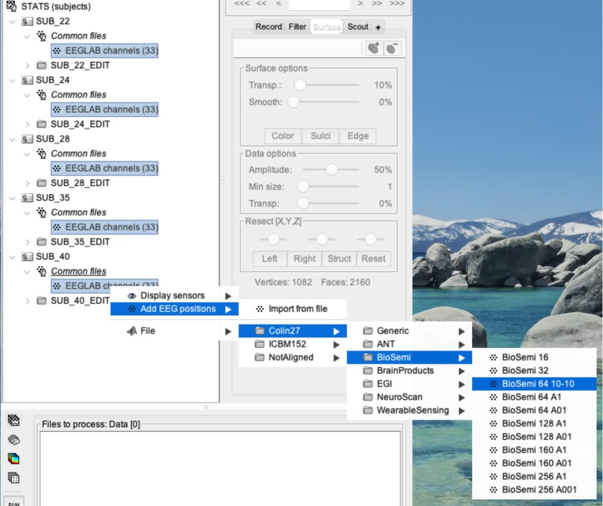
The screenshots in this problem set show an older protocol name (STATS). Name yours ProblemSet5.
c)Switch the database view to the middle icon (functional data sorted by subjects), as in PS1.
d)Create 10 subjects named to match your files:
SUB_6, SUB_7, SUB_8, … SUB_15 (right-click ProblemSet5 > New subject > type the name > Save).
e)Import each subject’s data:
right-click the subject (e.g., SUB_6) > Import MEG/EEG
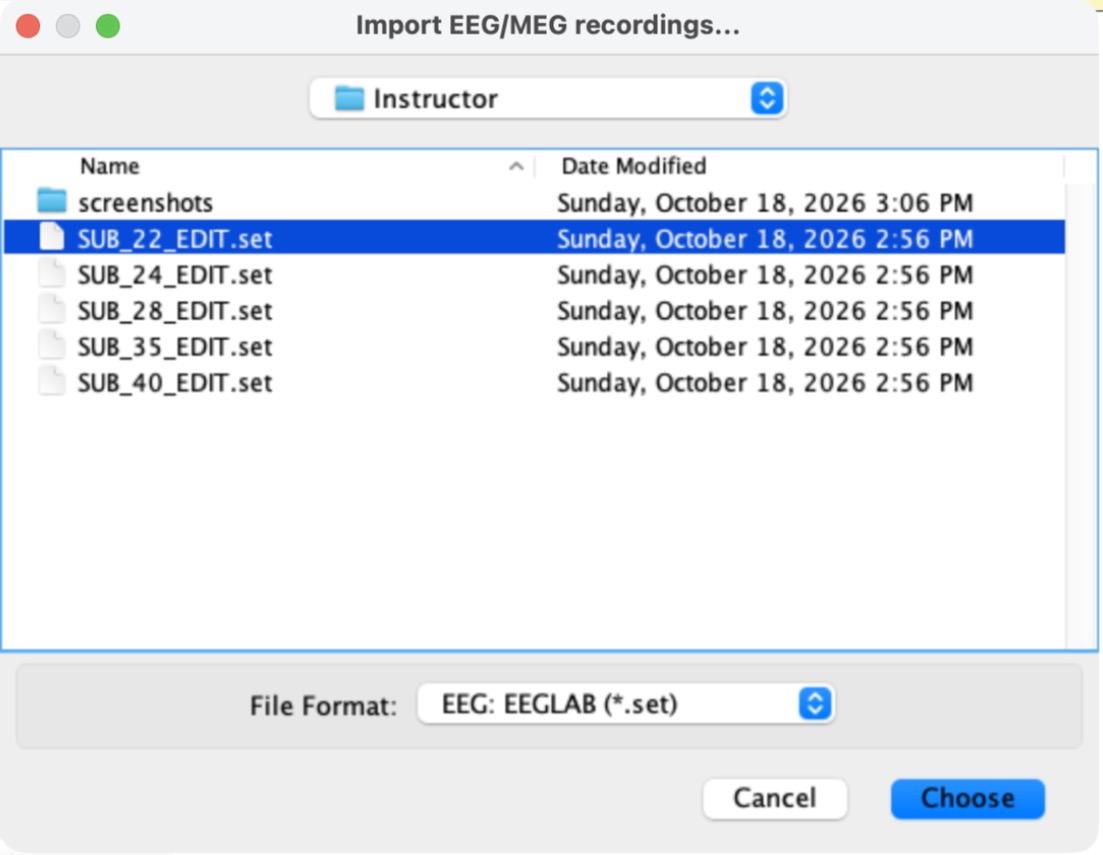
i)Change the File Format to “EEG: EEGLAB (*.set)” (it is far down the list), then select that subject’s _EDIT file and click Choose. Make sure the file matches the subject: SUB_6_EDIT.set goes into SUB_6, SUB_7_EDIT.set into SUB_7, and so on.
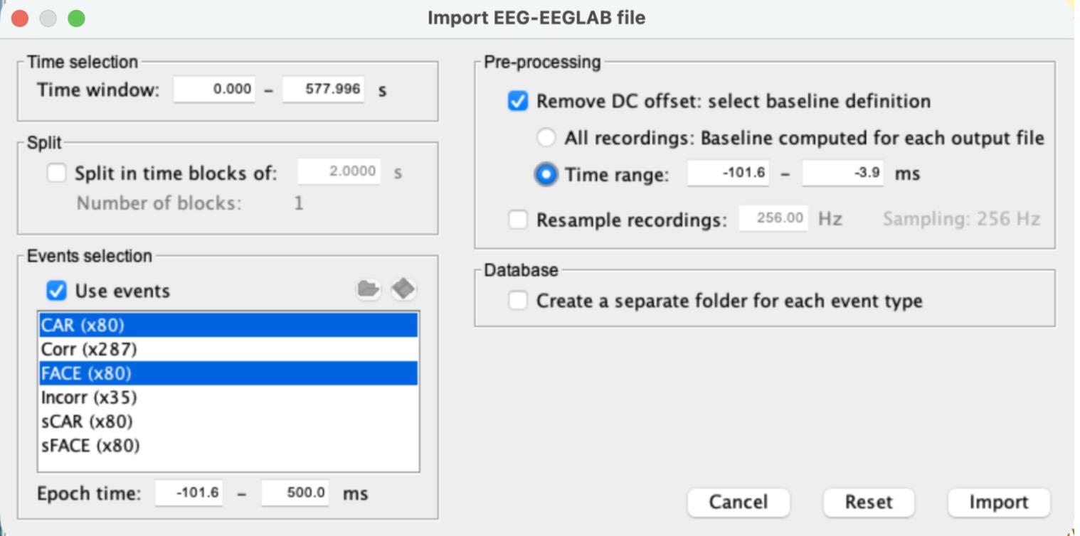
ii)In the import window, check “Use events” and select both CAR and FACE (Cmd-click on a Mac, Ctrl-click on Windows).
iii)Set the Epoch time to -100 to 500 ms. Brainstorm will adjust it to -101.6 to 500.0 ms.
iv)Check “Remove DC offset” and choose “Time range”. Brainstorm fills in about -101.6 to -3.9 ms (the period before the picture appears). Leave “Create a separate folder for each event type” unchecked. Your settings should match the picture below. Click Import.
v)Repeat for all 10 subjects. Brainstorm usually remembers your last settings, but check every time that CAR and FACE are both selected and “Remove DC offset” is checked.
Note: MATLAB’s Command Window will fill up with lines like “EEGLAB> Warning: ICA matrices are present in the file, but ignored in Brainstorm.” That is expected; you can ignore it.
2)Edit the EEG positions for all subjects at once
a)Expand each subject and its “Common files” folder so you can see every “EEGLAB channels (33)”.
b)Select all 10 “EEGLAB channels (33)” files (Cmd-click / Ctrl-click), then right-click > Add EEG positions > Colin27 > BioSemi > BioSemi 64 10-10.
c)A summary window lists each subject (“28 channels updated, 0 channels not found”).
Click OK. If a subject is missing from the list, repeat this step for that subject.
3)[0.5 pts] Create subject ERPs
a)Change to the third icon (functional data sorted by conditions).
Each subject’s data folder (SUB_6_EDIT, SUB_7_EDIT, …) is now listed in the tree.
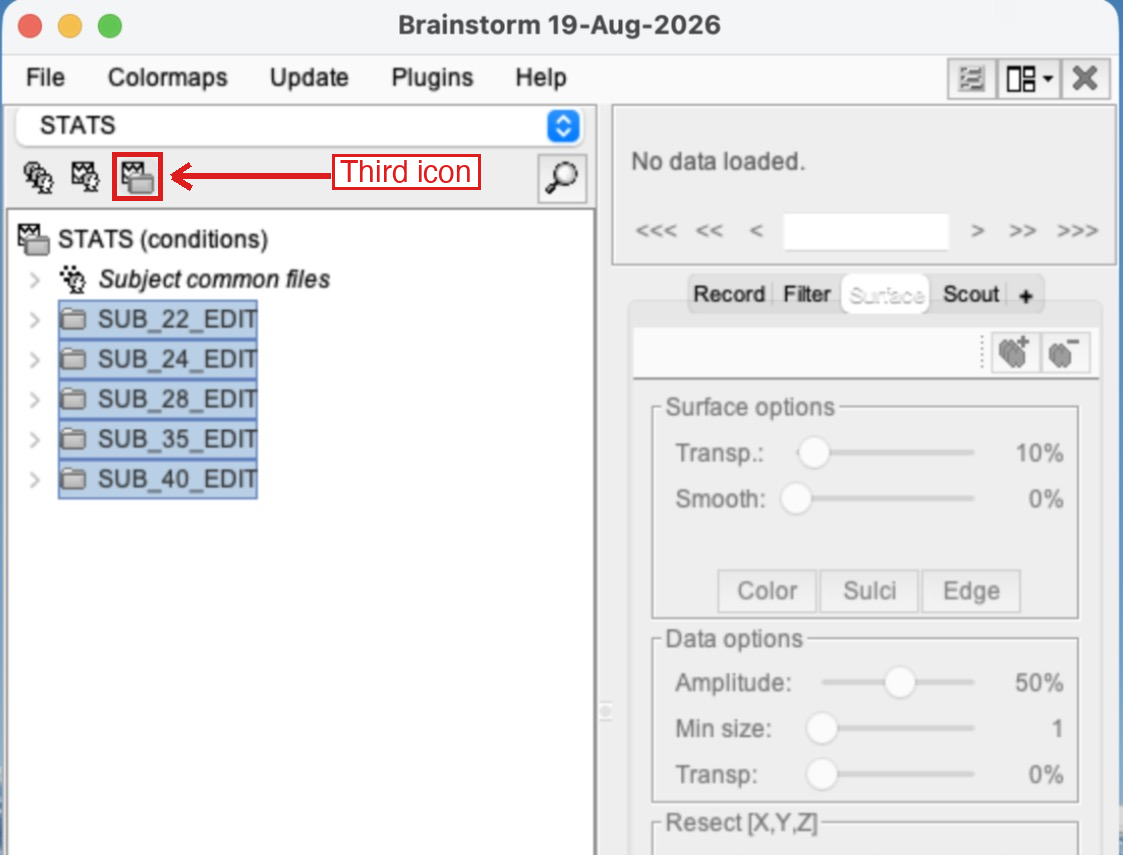
b)Select all 10 data folders (click the first one, then Shift-click the last one) and drag and drop them into the “Files to process” panel at the bottom.
It should say Data [1600] (10 subjects × 160 trials).
c)Click RUN.
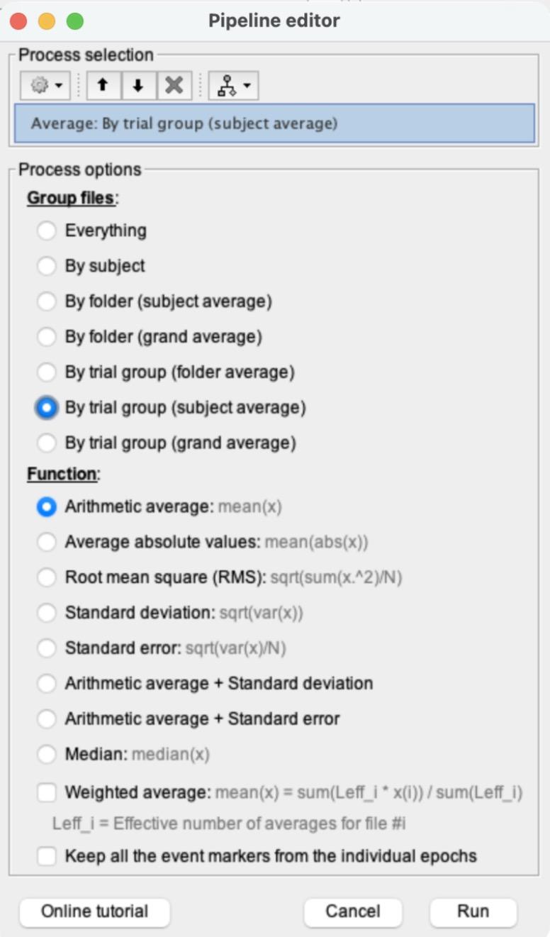
In the Pipeline editor, click the gear icon (Add process) > Average > Average files.
d)Choose “By trial group (subject average)” and “Arithmetic average”, then click Run.
This creates 2 ERPs for each subject, “Avg: FACE (80 files)” and “Avg: CAR (80 files)”, inside each subject’s folder.
e)Expand SUB_9_EDIT > SUB_9 and double-click “Avg: FACE (80 files)”. Make sure the plot is in butterfly mode (it usually opens that way; if not, use the Display configuration button on the right). Click the channel with the most noticeable N170 (the biggest negative dip between about 130 and 170 ms) to highlight it in red, then click at the bottom of that dip to place the red vertical time marker. Take a screenshot with the time point visible in the top left, and say which channel you chose.
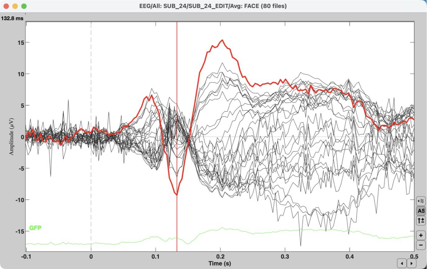
Example from the instructor demo subject (SUB_24). Your plot for SUB_9 will look different.
Tip: if the axis numbers look tiny, switch the plot to Column mode and back to Butterfly mode. This is a display glitch in MATLAB 2026.
4)[0.7 pts] Create group ERPs
a)Clear the “Files to process” panel (right-click inside it > Clear list).
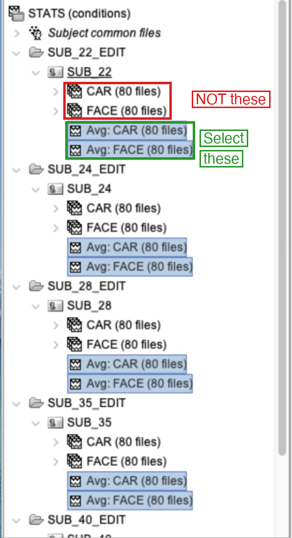
b)Select all 20 subject-average ERPs:
“Avg: FACE (80 files)” and “Avg: CAR (80 files)” in every subject (Cmd-click / Ctrl-click).
i)Select the Avg (ERP) files, NOT the “FACE (80 files)” / “CAR (80 files)” groups of individual trials!
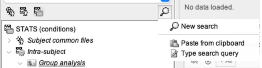
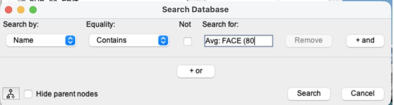
ii)Tip (optional): instead of clicking 20 files, let Brainstorm find them. Click the magnifier icon at the top right of the file list > New search. Leave “Name” and “Contains”, type Avg: in “Search for”, and click Search. A new tab opens that shows only files whose name contains “Avg:”. Drag the top line of that tab (ProblemSet5) into “Files to process”. Afterwards, close the search tab with the x on the tab to get the full file list back.
This example searches for Avg: FACE (80, which you will use in step 7. Here, type Avg: instead.
c)Drag and drop them into “Files to process” (it should say Data [20]) and click RUN.
d)Add process > Average > Average files.
Choose “By trial group (grand average)” > Run.
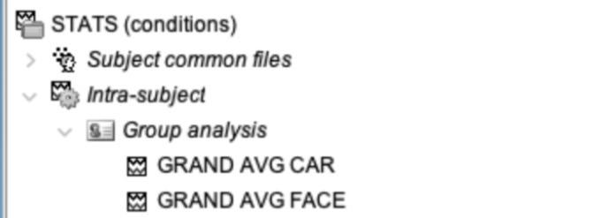
e)A new “Intra-subject” entry appears near the top of the tree.
Expand Intra-subject > Group analysis and rename the two new files, “Avg: Avg: FACE (10 files)” and “Avg: Avg: CAR (10 files)”, to GRAND AVG FACE and GRAND AVG CAR. (Right-click > File > Rename, or select the file and press F2.)
Instructor demo shown (5 subjects). You will have 10.
f)Double-click GRAND AVG FACE to plot it in butterfly mode.
i)Take a screenshot.
ii)How does this compare to the subject-average FACE ERP from step 3e? Focus on what you notice about the activity in the baseline period (before 0 ms).
5)[0.5 pts] Create a single combined average of the two grand-average ERPs
a)Clear the “Files to process” box.
b)Drag both GRAND AVG files into “Files to process” and click RUN.
c)Add process > Average > Average files.
Select “Everything” as the grouping option and leave the function as Arithmetic average > Run.
d)A new file appears under Group analysis.
Rename it “Avg of FACE and CAR”.
e)Double-click it to plot it.
Switch to column mode and highlight the channels where the N170 is typically most pronounced (think back to earlier problem sets, or to the channel you picked in step 3e). Cmd-click / Ctrl-click to highlight several channels.
f)Take a screenshot of the highlighted channels in column mode.
g)With these channels still highlighted, press Enter.
A new plot opens with only your channels (just like in PS1 and PS3). Switch the new plot to butterfly mode so the lines overlap, find the time point where they reach their most negative N170 peak, and click there to place the time marker.
i)Take a screenshot of the new plot with your selected time point clearly visible in the top left corner.
ii)Write this time down. We will call it your “N170 peak time.”
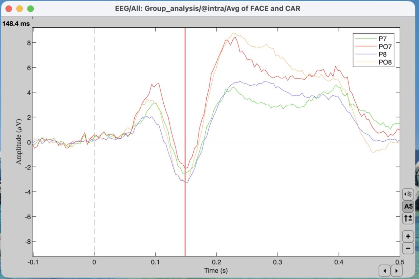
Instructor demo: P7, PO7, P8 and PO8 highlighted, then Enter. Your channels and time may differ.
Brief Note on Difference Waves:
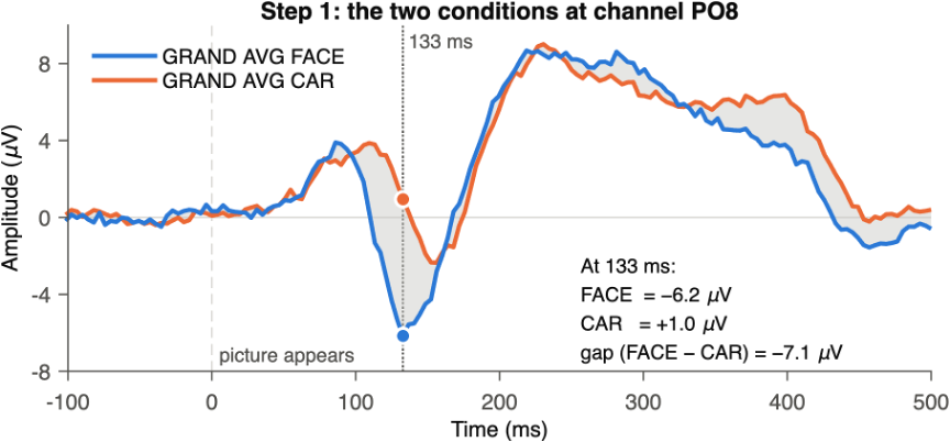
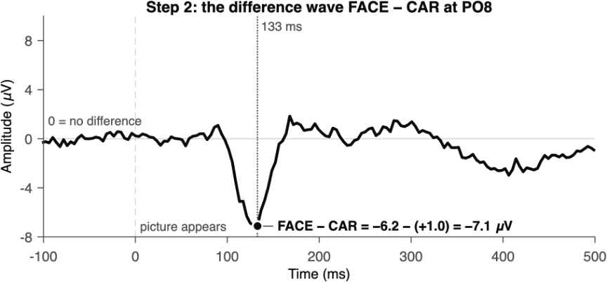
A difference wave is one ERP subtracted from another, point by point. At every time point (and at every channel), you take the value for condition A and subtract the value for condition B. The result is a single waveform that shows only how the two conditions differ.
Why it is useful:
1.It isolates the effect. Activity that is the same in both conditions (the early P1 to any picture, the general response to seeing something on the screen) cancels out. What is left is the part that is specific to faces.
2.Zero has a meaning. 0 µV means “no difference.” Below zero, FACE is more negative than CAR; above zero, FACE is more positive. Before the picture appears, the difference wave should hover around 0, because nothing about the two conditions differs yet.
How it is made:
6)[0.7 pts] Create a difference wave & visualize the N170 effect
a)Close the plots from step 5 and return to the main Brainstorm window.
b)Click “Process2” at the bottom of the Files to process panel.
You will now see two panels, Files A and Files B.
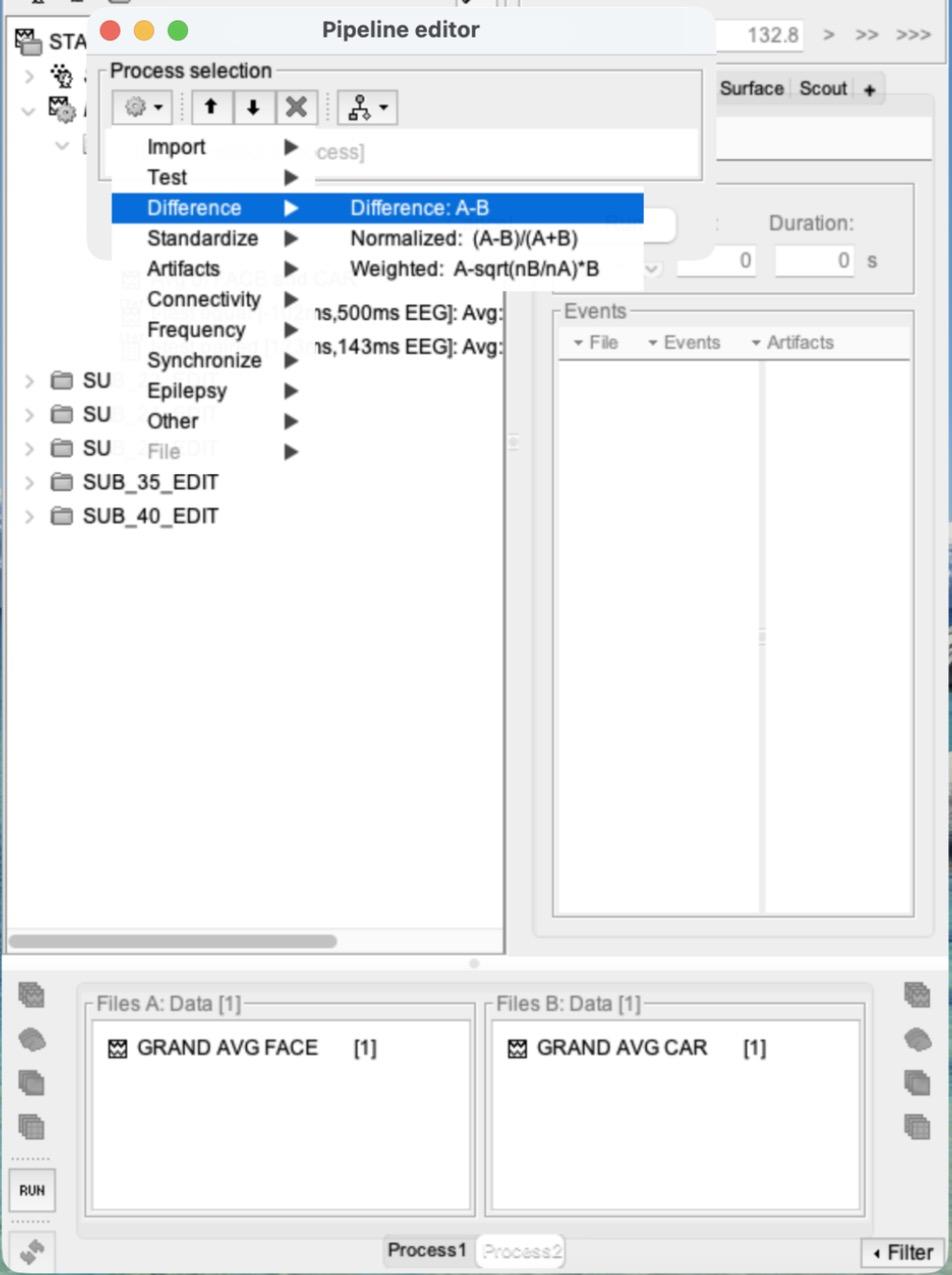
c)Drag GRAND AVG FACE into Files A and GRAND AVG CAR into Files B.
d)Click RUN > Add process (gear icon) > Difference > Difference:
A-B > Run. This creates “GRAND AVG FACE - GRAND AVG CAR”, the FACE minus CAR difference wave.
e)Plot the ERP waveform:
double-click the difference wave and put it in column mode. Set the y-axis scale to about -7 to 7 μV. Find the N170 effect: the most negative point of the difference wave in channels P8, PO8 and O2 (hint: it is earlier than 170 ms, and earlier than your N170 peak time from step 5). Click there to place the red time marker.
f)Plot channel PO8 separately:
highlight only PO8 in the difference-wave plot and press Enter. (Switch back to column mode if you can’t find it.)
g)Plot the scalp topography:
in the database tree, right-click the difference wave > EEG > Display on scalp. Then right-click the scalp plot > Channels > Display sensors, and right-click > Channels > Display labels. The head opens viewed from the top; click and drag to rotate it so you can see the back of the head, where the N170 is.
h)Take a screenshot of the three plots from 6e, 6f and 6g together, with the time marker visible in the top left of the waveform plot.
i)Write down this time. We will call it your “N170 effect time,” and you will use it in steps 7 and 8.
Think about it: why does the FACE − CAR difference peak earlier than the N170 itself? (Hint: compare when the FACE and the CAR N170 each reach their most negative point.)
7)[0.5 pts] Paired t-test at every time point (mass univariate)
a)Clear the Files A and Files B panels (right-click inside each > Clear list).
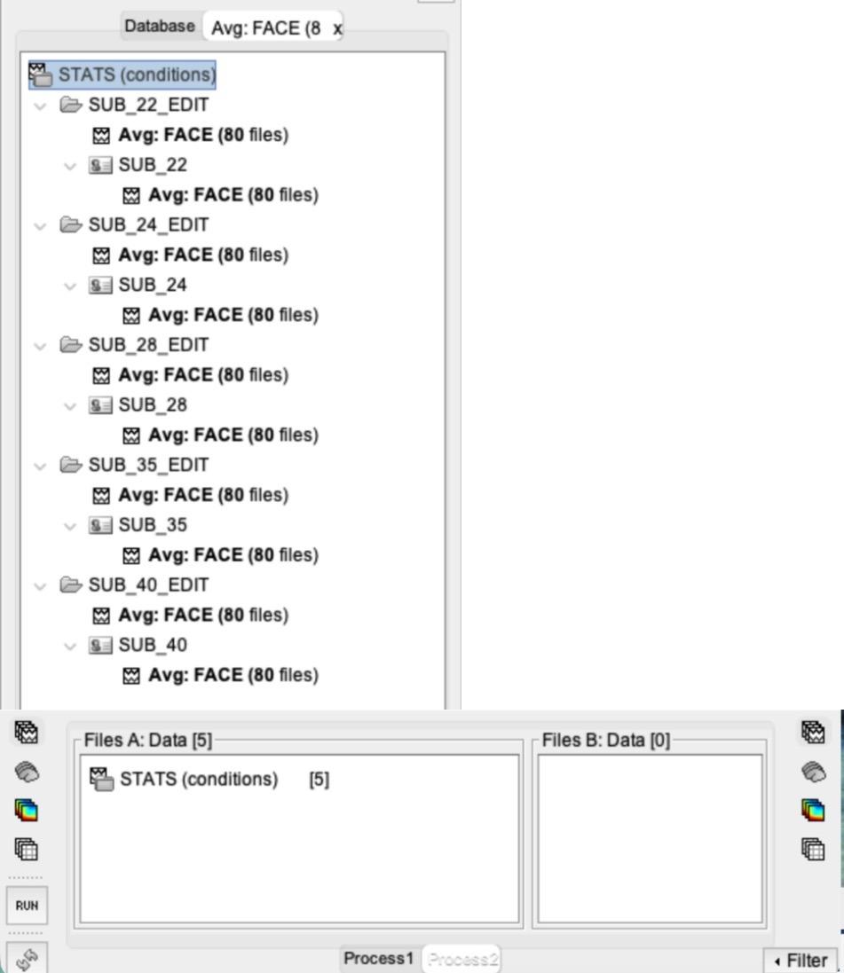
b)Select all 10 subject-average FACE ERPs (“Avg:
FACE (80 files)”, NOT the grand average) with Cmd-click / Ctrl-click, then drag and drop them into Files A.
i)Drag and drop them ALL AT ONCE. Don’t drag and drop one file at a time!
ii)Or use the search from step 4b: search for Avg: FACE (80 and drag the top line of the search tab into Files A. Then close the search tab.
Instructor demo (5 subjects): each file is listed twice in the search tab, but only 5 are added.
c)Repeat for all 10 CAR ERPs (“Avg:
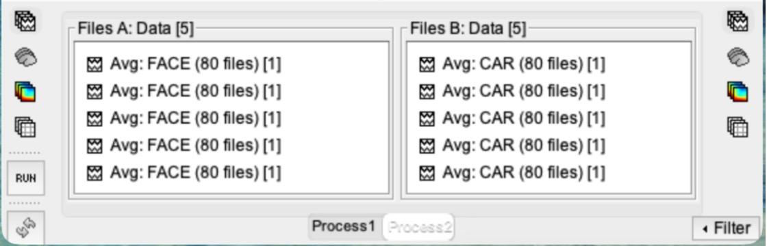
CAR (80 files)”, or search for Avg: CAR (80) into Files B. Each panel should say Data [10].
Instructor demo shown (5 subjects). You will have 10 in each list.
d)Click RUN > Add process > Test > Parametric test:
Paired.
e)UNcheck “Average selected time window”, type EEG in “Sensor types”, and keep “Two-tailed”.
Click Run.
This creates “t-test paired [-102ms,500ms EEG]: Avg: FACE vs. Avg: CAR (10)” under Intra-subject > Group analysis. Double-click it to plot it.
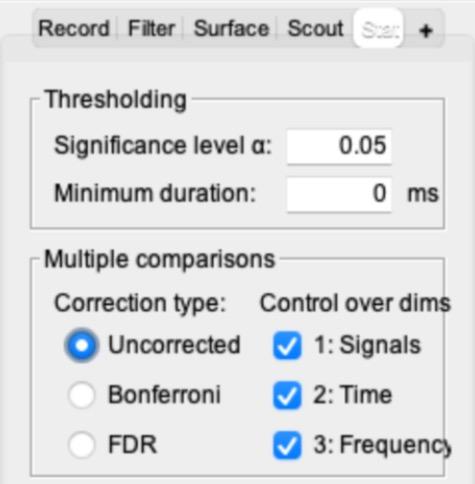
f)In the main Brainstorm window, open the “Stat” tab (it appears next to Record / Filter / Surface / Scout once a t-test is open).
Set Multiple comparisons to “Uncorrected” and check that the significance level α is 0.05. Brainstorm starts on “FDR”, which can hide results, so the plot may look different until you change this.
Why “Uncorrected”?
This ran a separate t-test for every channel at every time point: 28 × 155 = 4,340 tests. At α = 0.05, about 1 in 20 tests comes out “significant” by chance even when nothing is there, so expect some scattered significant blips. You will learn how to correct for this (FDR) in lecture and use it in Problem Set 6.
g)Right-click the t-test > EEG > 2D Disc.
Then right-click the disc > Channels > Display sensors, and right-click > Channels > Display labels. Resize the windows so both plots are visible.
h)Place your time marker at your N170 effect time from step 6 (not the step 5 time) and take a screenshot of both plots together. Which electrode(s) show a significant difference between faces and cars?
8)[0.5 pts] Paired t-test on mean amplitude, compared with an independent t-test
a)Close all figure windows (this will save your in-progress work from those images).
You can also type ‘close’ into the matlab command window to close all windows except the GUI.
b)Keep the Files A and Files B lists from step 7.
Click RUN again.
c)Add process > Test > Parametric test:
Paired.
d)Type EEG in “Sensor types” and CHECK “Average selected time window”.
For the Time window, enter your N170 effect time from step 6 plus/minus 10 ms. Click Run. Note that this is the N170 effect time you found from the difference wave, not the N170 peak time from Step 5.
i)For example, if your N170 effect time was 130 ms, use 120 ms to 140 ms.
ii)Brainstorm will adjust these slightly; it doesn’t need to be exact.
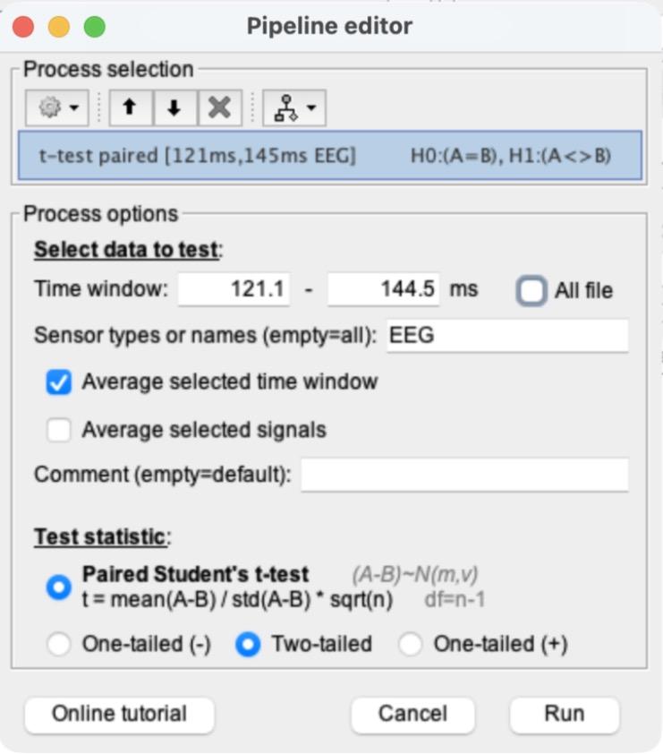
e)This creates “t-test paired [xxx ms, xxx ms EEG]:
…” under Intra-subject > Group analysis.
f)Right-click the new paired t-test > Display as image.
Then right-click it again > Display as table. The table lists each channel’s t-value; the two columns are the start and end of your time window and show the same value. A 0 means that channel is not significant at α = 0.05.
Instructor demo’s table (5 subjects). Your values will differ.
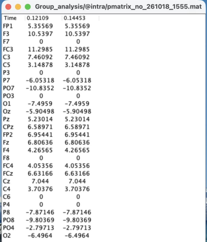
g)Take a screenshot of the image and the table, and explain what this result indicates.
h)For comparison, run an independent t-test on the same data.
With Files A and B unchanged, click RUN > Add process > Test > Parametric test: Independent. Use the same settings as 8c (EEG, “Average selected time window” checked, the same time window) and click Run. Right-click the new “t-test equal […]” file > Display as table.
i)Compare the two tables. Which electrodes are significant in the paired test but not in the independent test? Every subject saw both faces and cars. Why does that make the paired test the right one here, and why does it find more?
Think about it:
in a real study, the time window is chosen before looking at the data (the ERP CORE study used 110–150 ms), so you are not just picking whatever window looks best.
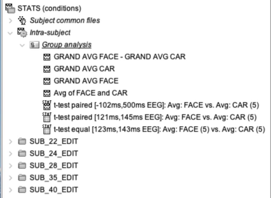
9)[0.3 pts] At the end, take a screenshot of the expanded “Intra-subject” section in your Brainstorm window, showing all of the GRAND AVG files, the GRAND AVG difference wave, and all three t-tests.
a)You may need to drag the divider to the right of the file tree to widen it.
We don’t need to see the whole name, but we should be able to tell what each file is.
Instructor demo shown.